Optimal routes project
Summary
The present s web site is the result of the process carried out by the optimal routes team, which summarizes the work developed by a multidisciplinary group of professionals in 2020 and which was led by the Statistical Research Subdepartment. This process resulted in the document entitled Rutas optimas para recolectores del IPC of which the document presented below is its applied part. The next process describe the choice of a genetic algorithm that allows ordering the proximity between the nodes and drawing the route that an IPC collector must follow over the assigned places. This implementation was statistically significant and the reduction in travel times was 15% in a total of 161 points in space.
We will use genetic algorithms (GA) to solve the street vendor problem. We will incorporate this method that uses an iterative process of 100 genetic algorithm solutions. Therefore, we will select the best of all those processes to solve a simple TSP with 10 spatial points. We also have that the AG are an optimization method or search algorithm. In this sense, a search algorithm can exhibit heuristic behavior if it is executed continuously, adapting to the dynamics of the environment in which it is used, thus exhibiting a learning behavior.
The process of generating optimal routes is illustrated using the R1 Through the use of a genetic algorithm (GA) created through the GA^library [Scrucca, L. (2012). GA: A Package for Genetic Algorithms in R. Submitted to Journal of Statistical Software], which is applied through a series of one hundred simulations from which the one that converges to an optimum is chosen. The application of the AG is estimated on a matrix of geographical distances from which the route that runs through the streets of Chile is built through an Open Source Route Engine (OSRM2) originally programmed in C ++ and implemented on a Docker container3 which was implemented via command line in the Terminal of the Linux Ubuntu operating system4 in the search for solutions to routes or routes for data collectors in the field.
Introduction
Originally known as the traveling salesman problem (TSP for short), the idea is to find the cheapest way to visit all the places and return - or not - to the starting point. The way to visit all the places is simply the order in which these points are visited, the route is called a tour or circuit through these points, as defined by Flood (1956).
This modest-sounding exercise is in fact one of the most intensely investigated problems in computational mathematics, says Little et al. (1963). It has inspired mathematical, computer, chemical, physical studies, and a wide variety of investigations. Teachers in some colleges around the world use the TSP to introduce discrete mathematics in elementary, middle and high schools, as well as universities and vocational schools. The TSP has had applications in the areas of logistics, genetics, manufacturing, telecommunications, and neuroscience, to name just a few disciplines, according to Applegate et al. (1998).
On the other hand, Jaffee (1996) states that the appeal of the TSP has elevated it to one of the few contemporary problems in mathematics to become part of popular culture. Its interesting name has surely played a role, but the main reason for the great interest is the fact that this easy-to-understand model still eludes a blanket solution. The TSP’s simplicity, coupled with its apparent intractability, makes it an ideal platform for developing ideas and techniques for tackling computational problems in general.
Brief history of TSP
The origin of the name “traveling salesman problem” is mysterious. There does not appear to be any documentation pointing to the originator of the name, and it is unknown when it first came into use. One of the first TSP researchers and one of the most influential was Merrill Flood in the US. However, there are also previous records in Germany and Switzerland regarding the same type of problem, according to Applegate et al. (2003).
In the 1950s, the name TSP was widely used. The first reference to the term appears to be a 1949 report, “On the Hamiltonian Game (A Traveling Salesman Problem)”, but it seems clear from the writing the name was not being introduced. However, it is possible to mention that sometime during the 1930s or 1940s, most likely in Princeton, the TSP took its name and mathematicians began to study the problem seriously, according to Applegate et al. (2003).
Some historical records obtained from Applegate et al. (2003) show how striking the traveling salesman problem is:


Genetic algorithm
The underlying idea of an algorithm is a series of organized steps that describes the process that must be followed to solve a specific problem. In the 70’s, from the hand of John Henry Holland, one of the most promising lines of artificial intelligence emerged, that of genetic algorithms, (AG). They are so called because they are inspired by biological evolution and its genetic-molecular basis (Mirjalili (2019)). These algorithms make a population of individuals evolve (for this particular case, tours) subjecting it to random actions similar to those that act in biological evolution (mutations and genetic recombinations), as well as to a selection according to some criteria, depending on from which it is decided which routes are more adapted, which “survive,” and which are the least suitable, which are discarded.
Charles Darwin once said in his book, The Origin of Species: “It is not the strongest of species that survives, nor the most intelligent, but the one that best responds to change” Darwin (1859). In this sense, we must understand the concept of “evolution” in the context of machine learning and thus understand the operating mechanism of this algorithm.
Therefore, the genetic algorithm is an adaptive procedure based on the mechanisms of natural genetics and natural selection. The genetic algorithm has two essential components: survival adjustment and genetic diversity. Originally developed by Holland (1975), the Genetic algorithm (GA) is a heuristic search that is assimilated to the process of natural evolution. Use the concept of “Natural Selection” and “Inherent Genetics” from Darwin (1859). Currently there are an infinity of applications of Genetic algorithms such as optimization and resolution of scheduling problems, airspace engineering, astronomy and astrophysics, chemistry, electrical engineering, financial markets, materials engineering, molecular biology, pattern recognition and data mining robotics, just to name a few areas where it applies.
In our case, the genetic algorithm (GA) is used to solve the TSP. However, we add an additional component. That is, we generate 100 simulations of genetic algorithms that search for solutions, which are then contrasted and the answer that is repeated the most times in the total of simulations is selected, in order to obtain the best possible result. This additional component gives the learning character to the solution search process.
Operation in R
R Core Team (2020) is the project that supports the Statistical Software R, in which there is a whole work scheme that allows the creation of a clean implementation process of the traveling salesperson problem. This process begins with reading the libraries that allow us to work with databases (Wickham and Bryan (2019), Wickham et al. (2020) and Bittinger (2020)) and spatial databases (Bivand, Pebesma, and Gomez-Rubio (2013) and Pebesma (2018)) on the one hand and on the other, a set of libraries that allow us to process spatial information through the genetic algorithm (Scrucca (2012)) and create and map the resulting path (Giraud (2020) and Cheng, Karambelkar, and Xie (2019)). First of all, a crucial aspect is the implementation of an operating system Linux Ubuntu (Raggi, Thomas, and Van Vugt (2011)) that allows us to implement an open source routing engine (project OSRM, Huber and Rust (2016)) which, in turn, forces us to run a Docker (Boettiger (2015)). To know the benefits of working with containers and especially Docker, it is recommended to review general aspects on the application website.
Therefore, we must have access to a set of elements necessary to execute the process. The necessary components are: an operating system Linux-Ubuntu, R (with its libraries), Rstudio and OSRM implemented in a Docker container. The process is made up of four stages; the first corresponds to the reading of the spatial databases, which allow the identification of the points of the places to visit, which must be correctly determined geospatially. In the case of Chile, these points are determined by properly implemented spatial standards, which in our case was the task of the Geography Department, who gave us the latitude and longitude points of each establishment. The second stage, corresponds to the processing of a distance matrix by means of a method that includes the participation of one hundred genetic algorithms. This process considers a combination of all the solutions from which the best answer is extracted; The third stage is the generation of the route product of the spatial order previously calculated by means of a route engine (OSRM) that will allow to use real data (from Open Street Map) known to move between one point and another; and the fourth and last stage is the mapping of the solution on an interactive map.
In this report, the geospatial determination will be carried out using the tmaptools library (Tennekes (2020)) through the geocode_OSM function, which uses the standard defined for data distributed through OSM (Bennett (2010)) and which can be reviewed in their official document5. In addition, the use that we will give we must comply with not over-demanding these servers that have a non-intensive use, since we could be blocked in case we make intensive use. On the other hand, in order to protect the information handled by our INE, we will use addresses and spatial points corresponding to non-sensitive sites and museums (10 in total) located in the center of Santiago. In this way, we avoid publishing information that may be private or sensitive and at the same time, we do not over sue the public servants of the OSM project6.
Routing Engine (OSRM)
A routing engine is a system that, from a list of ordered spatial points, returns a route through the streets, the type of transport, the time and the total distance traveled. Therefore, in the world of web mapping, the path to the reality of optimized route calculation is one of the great challenges. It is not only about going from point \(A\) to point \(B\), but about proposing several options, alternative itineraries, taking into account the different modes of transport (car, walk, train, bicycle, boat, etc.), include stages, respect the meanings of the streets. Thus, the emergence of mobile equipment reinforces the importance of these services, whose efficiency depends on the quality of the data used.
In this experience, Google Maps is not an option in a State institution. After investigating different alternatives, we opted for the idea of putting together an itinerary free engine, specific and very convenient for our reality, often limited in economic resources.
The schematic map that describes the deployment process considers work using the Linux Ubuntu 20.04 operating system (Petersen (2020)), which was later deployed on a Linux Centos server at the INE. This process first required the installation of the Docker tool (Boettiger (2015)), which is a container system that will allow to query (through a generated API) of the routes when the OSRM project software (Giraud (2020)) is launched. In this section, we detail the process used to assemble the routing engine.
OSRM project beginnings
In English Open Source Routing Machine (OSRM), it means that it is an open source routing machine and corresponds in other words to a routing server designed to be used with the data provided from the OpenStreetMap (OSM) project also from the world of free software.
The OSRM project showed its first fruits on July 9, 2010, built entirely by the work developed by Dennis Luxen. The following year, Luxen presented on OSRM at ACM’s GIS ’11 conference alongside Christian Vetter7 Currently the Mapbox routing team continues the project, maintaining and developing it (Detomasi, Mathieu, and Botto (2018)).
Characteristics
In contrast to most routing servers, OSRM (Giraud (2020)) does not use a variant of A* to calculate the shortest path, but instead uses collapse hierarchies. This results in very fast query times, typically under 1 millisecond for large data sets over a thousand nodes. This is why OSRM is a good candidate for responsive web-based routing sites and applications. Their characteristics are:
- Very fast routing
- Highly portable
- Simple data format that facilitates custom import of data sets instead of OpenStreetMap data or import of traffic data
- Flexible routing profiles (e.g. for various modes of transport)
- Interpret turn restrictions, including time-based conditional restrictions
- Interpret turn lanes
- Driving instructions located by OSRM
Services and applications that use OSRM
- ES:Cycle.travel – direcciones en bicicleta
- Maps.Me – direcciones y mapas móviles fuera de línea
- Las API asociadas a OSRM son usadas por varios servicios webs, tales como RunKeeper
- MapboxDirections.swift en las plataformas de Apple como iOS
- Mapbox Servicios de Java en Java SE y Android
- Mapbox JavaScript SDK en el navegador y Node.js
- Mapbox Unity SDK
Docker deployment
As always on these issues, Google Maps was one of the pioneers to propose an efficient service on a large scale. Your data and your service are related to a commercial and proprietary policy. Likewise, in other competitors: Bing Maps, Yahoo Maps, ArcGis, etc.
We were looking for a system that works independently and for free, so we have chosen OSRM (Open Source Routing Machine), which is based on OpenStreetMap (OSM) data. It is not the only solution that exists to calculate itineraries, but it is very simple to implement and above all it is very powerful. The official page of the project can be visited here [http://project-osrm.org/-lex.europa.eu(http://project-osrm.org/] Creado por Dennis Luxen del Instituto Tecnológico de Karlsruhe, OSRM (Giraud (2020)) es programado mayormente en C++ y compatible con la mayoría de los sistemas operativos (Linux, FreeBSD, Windows, Mac).
The OSRM is based on road data and the quality of this data will depend on the quality of the result. As always in spatial data, two points are important, geometry and attributes. Geometry is the most obvious thing to understand because it is visual and it is perfectly understood if a street is not present in our database, our algorithm will not be able to give us a route that passes through it. Regarding attributes, their role is different but their importance is the same. Indeed, a database that contains information (that is, fields) on the direction of traffic, the maximum authorized speed or the number of lanes will offer much more potential than one that contains only the geometry and names of the roads.
The advantage of open data goes ahead of the question of price (although it is not negligible when the important cost of a proprietary road database is known), but also with the philosophy of having the freedom to modify said codes if necessary. necessary, the option is always open. The OSM model works perfectly (you have to see the quantity and quality of data in Europe and the US), the best proof of that was from Google’s Map Maker which allows users to edit (add, delete, modify), now based on Google Maps data. The difference is that this data created by the user is the property of Google and not of it, nor of a community.
Docker in Ubuntu 20.04
First we must install the Docker software on our system, using the Linux Ubuntu system terminal for these purposes. To which, through said terminal, we can install Docker. The steps and the process consider the following stages.
Installation and commissioning
To install the Docker engine, we need a 64-bit version of Ubuntu, in our case Ubuntu 20.04. The Docker engine is supported on x86_64 (or amd64), armhf, and arm64 architectures. In this case we install using the repository.
Before installing the Docker engine for the first time on our host computer, we must define the Docker repository. Then we can install and update Docker from the repository.
Defining the repository
+ Update the apt package index and install the packages to allow apt to use the repository over HTTPS:$ sudo apt-get update
$ sudo apt-get install \
apt-transport-https \
ca-certificates \
curl \
gnupg-agent \
software-properties-commonAdding the official Docker GPG key
$ curl -fsSL https://download.docker.com/linux/ubuntu/gpg | sudo apt-key add -We verify that we now have the key with the fingerprint 9DC8 5822 9FC7 DD38 854A E2D8 8D81 803C 0EBF CD88, by verifying that the last 8 digits coincide.
$ sudo apt-key fingerprint 0EBFCD88

pub   rsa4096 2017-02-22 [SCEA]
      9DC8 5822 9FC7 DD38 854A  E2D8 8D81 803C 0EBF CD88
uid   [unknown] Docker Release (CE deb) <docker@docker.com>
sub   rsa4096 2017-02-22 [S]
Installing the Docker engine
- We updated the Ubuntu libraries, and install the latest version of the Docker engine.
 $ sudo apt-get update
 $ sudo apt-get install docker-ce docker-ce-cli containerd.io
Installation verification
- With the following command, we verify that the word “Hello-World” results.
$ sudo docker run hello-worldThis command downloads a test image and runs it in a container. When the container runs, it prints the informal message and exits.
The Docker engine is installed and running. The docker group is created but there is no user enrollment. We must use the sudo command to run Docker. We are continuing with the installation from Linux to allow non-privileged users to run Docker commands and for other optional configuration steps.
OSRM for maps of Chile
At this stage we must go to the website Github of project OSRM. Then using the Ubuntu terminal we must follow the steps.
Using Docker
We use Docker OSRM images (backend, frontend) on Debian and make sure they are as lightweight as possible.
We downloaded the maps of Chile from OpenStreetMap, for example, from Geofabrik. This map is regularly updated with the information provided by the Chilean community and that feeds these databases with geospatial information.
wget http://download.geofabrik.de/south-america/chile-latest.osm.pbf
We pre-process the extract with the profile and initialize a routing engine HTTP server on port 5000 with the following Docker command.
docker run -t -v "${PWD}:/data" osrm/osrm-backend osrm-extract -p /opt/car.lua /data/chile-latest.osm.pbfThe -v flag creates the “/data” directory inside the Docker container and makes it available there. The file “/data/chile-latest.osm.pbf” inside the container is referenced in “/chile-latest.osm.pbf” on the server.
We run
docker run -t -v "${PWD}:/data" osrm/osrm-backend osrm-partition /data/chile-latest.osrm
docker run -t -v "${PWD}:/data" osrm/osrm-backend osrm-customize /data/chile-latest.osrm
Note that chile-latest.osrm has a different file extension.
docker run -t -i -p 5000:5000 -v "${PWD}:/data" osrm/osrm-backend osrm-routed --algorithm mld /data/chile-latest.osrmWe make the queries on the HTTP server
Once the OSRM server is up and running to receive route queries. This is possible to use me through the R library called OSRM. In this case, we will consider some georeferenced points around the city of Santiago, which will serve as an example of the use of OSRM.
At this stage we load the libraries, define two addresses of INE and museums in Santiago, to then obtain the geographic coordinates through OSM and then build a data frame with said information.
# Loading libraries
library(tmaptools)
library(leaflet)
library(osrm)

# Adresses to geolocalte
museos<-c("Morande 801, Santiago, Santiago",
         "Paseo Bulnes 418, Santiago",
         "José Miguel de La Barra 650, Santiago,Región Metropolitana",
         "Matucana 501, Santiago",
         "Portales 3530, Santiago, Estación Central, Región Metropolitana",
         "Av Vicuña Mackenna 37, Santiago, Región Metropolitana",
         "Plaza de Armas 951, Santiago, Región Metropolitana",
         "José Victorino Lastarria 307, Santiago, Región Metropolitana",
         "Av. República 475, Santiago, Región Metropolitana",
         "Fernando Márquez de La Plata 0192, Providencia, Región Metropolitana")

# Getting lat and lon
# geodato<-geocode_OSM(museos)

# In order to avoid making many queries to the server.
# We will use an RDS file

geodato<- readRDS("geodatos.RDS")

# Creating a data.frame
locs<-data.frame(id=geodato$query, lat=geodato$lat, lon=geodato$lon)
First visualization of data in space.
library(htmlwidgets)
library(webshot)
library(leaflet)
# Visualizamos en el espacio la ubicación de los museos
m<-leaflet(data = locs) %>% addTiles() %>%
  addMarkers(~lon, ~lat, popup = ~as.character(id), label = ~as.character(id))
m
Mapa de los puntos sin optimizar
In Figure we visualize the points in space using the leaflet library. This function creates a map widget using htmlwidgets. The widget can be rendered in HTML pages generated from R Markdown, Shiny, or other applications.
By using the sf library we construct a dataframe type object with spatial attributes. At its most basic, an sf object is a collection of simple features that includes attributes and geometries in the form of a dataframe. In other words, it is a dataframe (or tibble) with rows of features, columns of attributes, and a special geometry column that contains the spatial aspects of the features. This format is required for use in OSRM.
# Building spatial object of 10 museums
library(sf)
locs <- structure(
  list(id=geodato$query,lon = geodato$lon,  lat = geodato$lat),
  class = "data.frame", row.names = c(NA, -10L))
Through the osrmRoute function we make a route without order, only to show the use of OSRM does not generate any type of route optimization.
# A route between museums is estimated using the osrmRoute function
ruta1 <- osrmRoute(loc = locs, returnclass = "sf")
plot(st_geometry(ruta1), col = "red", lwd = 2)
points(locs[,2:3], pch = 20, cex = 3)
text(locs[,2:3],as.character(row.names(geodato)), cex = .8, col="grey")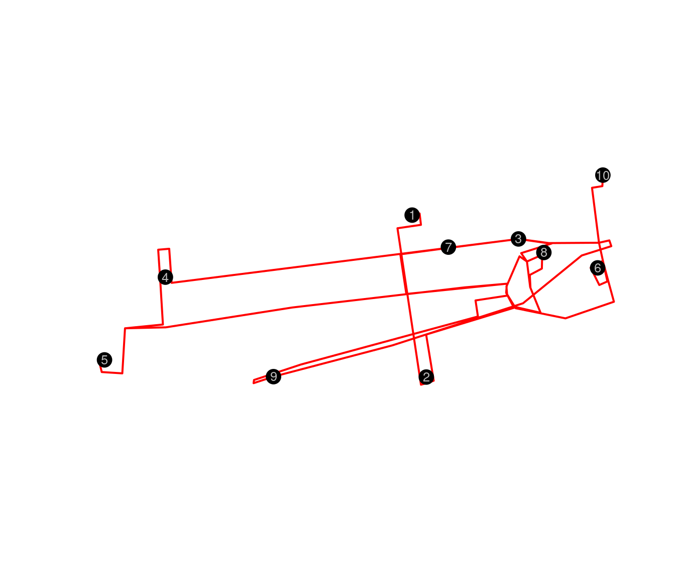
Ruta entre los museos sin optimizar
In Figure it is necessary to mention that this route does not have any type of optimization, since we only show the operation of OSRM, in this case there is no ordering.
We make the visualization for an interactive map visible in HTML.
library(htmlwidgets)
library(webshot)

# Same visualizatión, but in a interactive map.
m<-leaflet(data = sf::st_geometry(ruta1)) %>%
  setView(lng = mean(locs$lon), lat =mean(locs$lat), zoom = 14) %>%
  addTiles() %>%
  addMarkers(lng = locs$lon, lat = locs$lat, popup = locs$id) %>%
  addPolylines()
m
Mapa de los puntos sin optimizar
## Guardamos de html a png
#saveWidget(m, "temp.html", selfcontained = FALSE)
#webshot("temp.html", file = "Rplot.png",
#        cliprect = "viewport")
In Figure , it is evident that the interactive visualization using leaflet is a great advantage, since it allows us to build a final html file that is easy to use. automate and at the same time, convenient to share and view, and these can be used from mobile devices.
Genetic Algorithm on OSRM
Once we define that we will use the resolution advantages through AG, the mathematical process that will allow us to build the solution, we have to do the implementation.
An identifier with ID and names is added to the geodata object, if they exist, for the purpose of this exercise we are going to consider ID and names as equivalent. The distance matrix is built using the osrmTable function from the OSRM library, then it is transformed to a dist object of R, and then the names are added to said distance matrix.
#Building an ID
geodato$ID<-1:10
nombres<-1:10

# Building a matrix of distances
ma_dist <- osrmTable(loc = geodato[1:10, c("ID","lon","lat")])

# Object dist and naming points
bd<-as.dist(ma_dist$durations)
bd<-usedist::dist_setNames(bd, nombres)
The GA library is loaded to resolve the order of the tour. A seed is created and then said distance matrix is transformed into an R matrix type objective. The function that will measure the length of the tour, the adjustment function, the tour function, the coordinates through multidimensional scaling, are also created. the number of iterations with the corresponding matrix.
# We load the Genetic Algorithm library
library(GA)

# We define the random seed and bring it to an matrix
set.seed(123)
D <- as.matrix(bd)

# given a tour, we calculate the total distance
tourLength <- function(tour, distMatrix) {
  tour <- c(tour, tour[1])
  route <- embed(tour, 2)[, 2:1]
  sum(distMatrix[route])
}

# the inverse of the total distance is the setting
tpsFitness <- function(tour, ...) 1/tourLength(tour, ...)

# We create the tour function
getAdj <- function(tour) {
  n <- length(tour)
  from <- tour[1:(n - 1)]
  to <- tour[2:n]
  m <- n - 1
  A <- matrix(0, m, m)
  A[cbind(from, to)] <- 1
  A <- A + t(A)
  return(A)
}

# 2-d coordinates using multidimensional scaling
mds <- cmdscale(bd)
x <- mds[, 1]
y <- -mds[, 2]
n <- length(x)

# We define the number of iterations
B <- 100
fitnessMat <- matrix(0, B, 2)
A <- matrix(0, n, n)
We compile the results of the total iterations to later identify the most adjusted route. In addition, a meter of the total process time is added.
inicio1<-Sys.time()

for (b in seq(1, B)) {
  # ejecuta el AG
  AG.rep <- ga(type = "permutation", fitness = tpsFitness, distMatrix = D,
               min = 1, max = attr(bd, "Size"), popSize = 10, maxiter = 50,
               run = 100, pmutation = 0.2, monitor = NULL)

  tour <- AG.rep@solution[1, ]
  tour <- c(tour, tour[1])
  fitnessMat[b, 1] <- AG.rep@best[AG.rep@iter]
  fitnessMat[b, 2] <- AG.rep@mean[AG.rep@iter]
  A <- A + getAdj(tour)
}

final1<-Sys.time()
(final1-inicio1)
## Time difference of 9.178343058 secsA function is built to display the order of the tour in a distance matrix.
plot.tour <- function(x, y, A) {
  n <- nrow(A)
  for (ii in seq(2, n)) {
    for (jj in seq(1, ii)) {
      w <- A[ii, jj]
      if (w > 0)
        lines(x[c(ii, jj)], y[c(ii, jj)], lwd = w, col = "lightgray")
    }
  }
}
# We plot the points and the route fits between them
plot(x, y, type = "n", asp = 1, xlab = "", ylab = "", main = "Tour ordenado")
points(x, y, pch = 16, cex = 1, col = "blue3")
abline(h = pretty(range(x), 10), v = pretty(range(y), 10), col = "lightgrey")
tour <- AG.rep@solution[1, ]
#tour <- ruta[-11,1]
tour <- c(tour, tour[1])
n <- length(tour)
arrows(x[tour[-n]], y[tour[-n]], x[tour[-1]], y[tour[-1]],
length = 0.15, angle = 45, col = "green4", lwd = 2)
text(x+0.2, y+0.3 , nombres, cex = 1)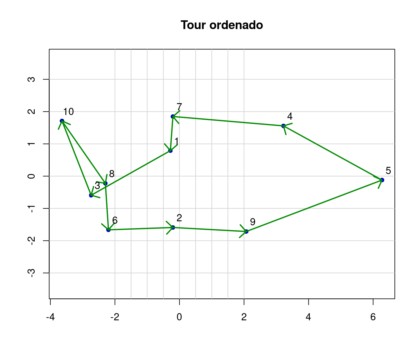
gráfico de los puntos y la mejor ruta que se ajusta entre los puntos
In Figure , the ordered tour for a field data collector is displayed. This tour is built based on the distance matrix.
# Summary of GA progression
summary(AG.rep)
## $type
## [1] "permutation"
##
## $popSize
## [1] 10
##
## $maxiter
## [1] 50
##
## $elistism
## [1] 1
##
## $pcrossover
## [1] 0.8
##
## $pmutation
## [1] 0.2
##
## $domain
## NULL
##
## $suggestions
## NULL
##
## $iter
## [1] 50
##
## $fitness
## [1] 0.03401360544
##
## $solution
## x1 x2 x3 x4 x5 x6 x7 x8 x9 x10
## [1,] 9 5 4 7 1 3 10 8 6 2
##
## attr(,"class")
## [1] "summary.ga"plot(AG.rep, main = "progresión de AG")
points(rep(30, B), fitnessMat[, 1], pch = 16, col = "lightgrey")
points(rep(35, B), fitnessMat[, 2], pch = 17, col = "black")
title(main = "50 primeras iteraciones sobre el total de 100 simulaciones
(mejor y promedio)")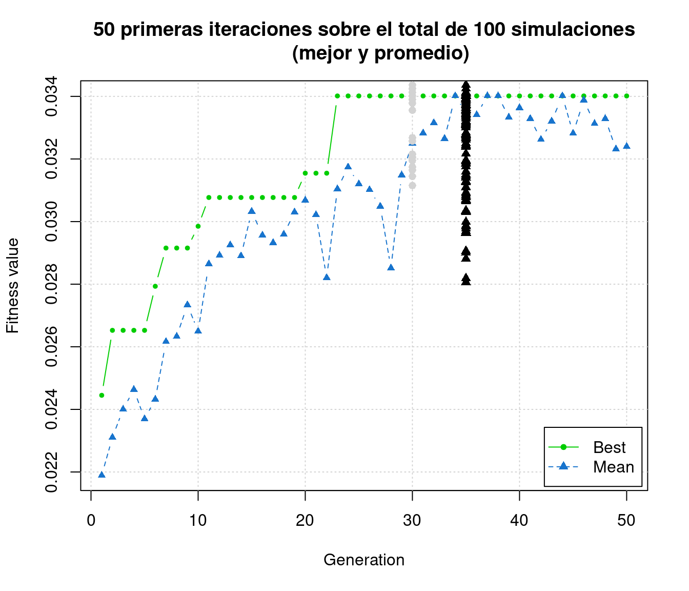
50 primeras iteraciones sobre el total de 100 simulations (mejor y promedio)
In Figure , we visualize the first 50 iterations. The graph describes the value of fitness or adjustment of the function of the genetic algorithm as a function of the number of generations. In this case we did a total of 100 simulations. It is important to note that when we construct the object AG.rep by function ga the argument maxiter = 50 was used, in order to define the total number of iterations for each genetic algorithm. Therefore, the average and the best of those 100 simulations are shown here, the ones that tend to converge between generation 30 and 40. This process is what gives a learning behavior to this solution.
plot(x, y, type = "n", asp = 1, xlab = "", ylab = "",
main = "Final route selected
      (100 simulations)")
plot.tour(x, y, A * 10/max(A))
points(x, y, pch = 16, cex = 1.5, col = "blue")
text(x, y, nombres, cex = 1)
lines(x[tour], y[tour], col = "red", lwd = 1)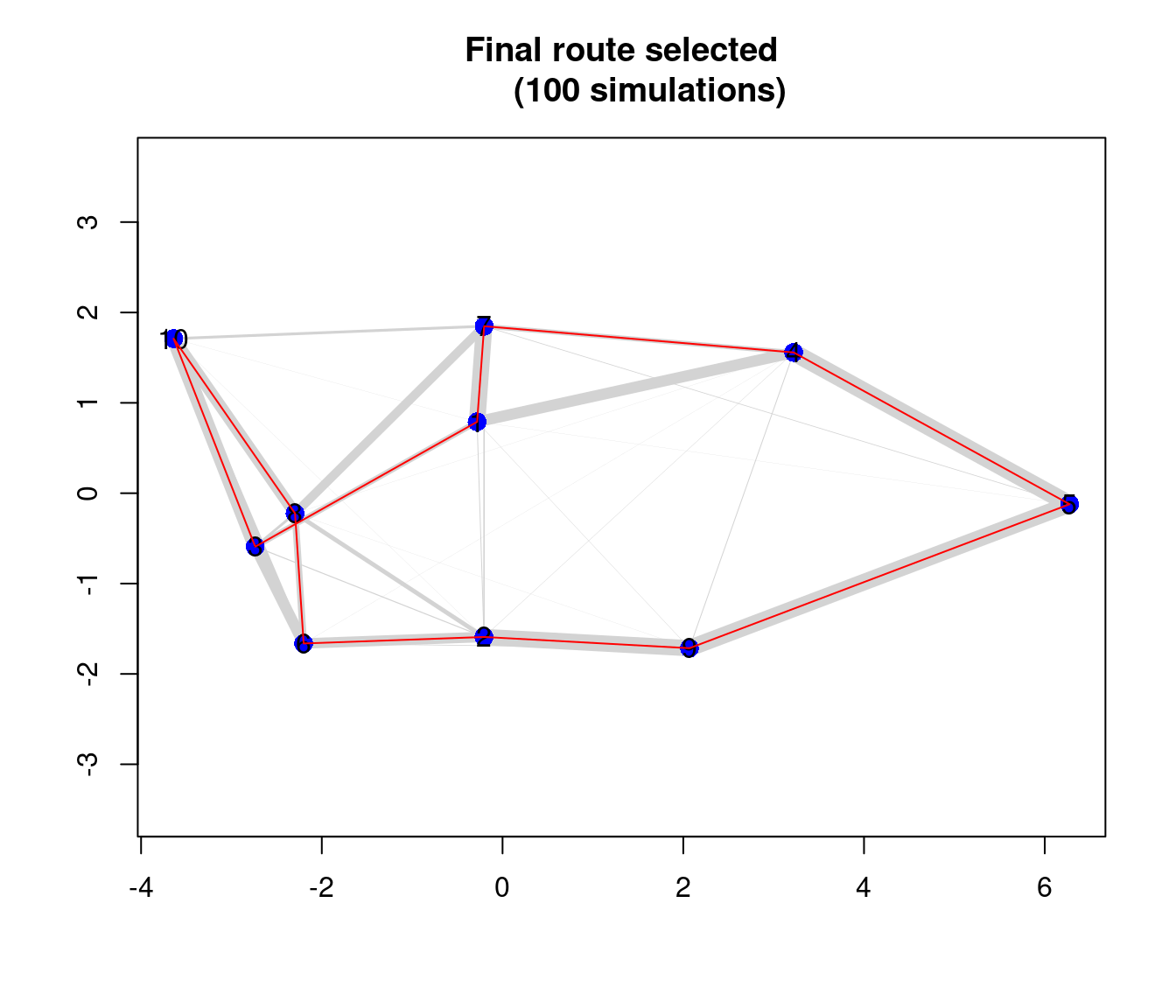
Gráfico del resultado de la mejor ruta
In Figure , we visualize the final selected path in red. In this graph it is possible to visualize in gray color it represents the proportion of the routes tested in the total of 100 simulations. Therefore, the width of the path between the points indicates how efficient that route was.
At this stage we obtain the solution and compare it with the tour solution in order to validate the results. Therefore, both must have the same order.
# Construction of the resultant vector
nombres_ordenados<-summary(AG.rep)$solution

#nombres_ordenados <- vector("character", 10L)
 #ordenamiento del vector
for (i in 1:length(tour[-11])){
  nombres_ordenados[i] <- print(nombres[tour[-11][i]])
}
## [1] 9
## [1] 5
## [1] 4
## [1] 7
## [1] 1
## [1] 3
## [1] 10
## [1] 8
## [1] 6
## [1] 2# data frame creation and verification
posiciones<-data.frame(tour=tour[-11], ID=as.numeric(nombres_ordenados))
#ordering of entry points
library(dplyr)
options(digits=10)
bd3<-left_join(posiciones, geodato, by="ID")At this stage we load the osrm library and then make the connection with the osrm server where we have implemented the route engine (OSRM) through Docker.
# osrm library load
library(osrm)
#options(osrm.server = "http://127.0.0.1:5000/")
locs <- structure(
  list(id=bd3$ID,lon = bd3$lon,
       lat = bd3$lat),
  class = "data.frame", row.names = c(NA, -10L))
Again a route is estimated spatially between the points using the osrmRoute function of the route engine. In this case, the ordering delivered is defined by the previously executed optimization process.
ruta1 <- osrmRoute(loc = locs, returnclass = "sf")
plot(st_geometry(ruta1), col = "red", lwd = 2)
points(locs[,2:3], pch = 20, cex = 3)
text(locs[,2:3],as.character(row.names(geodato)), cex = .8, col="grey")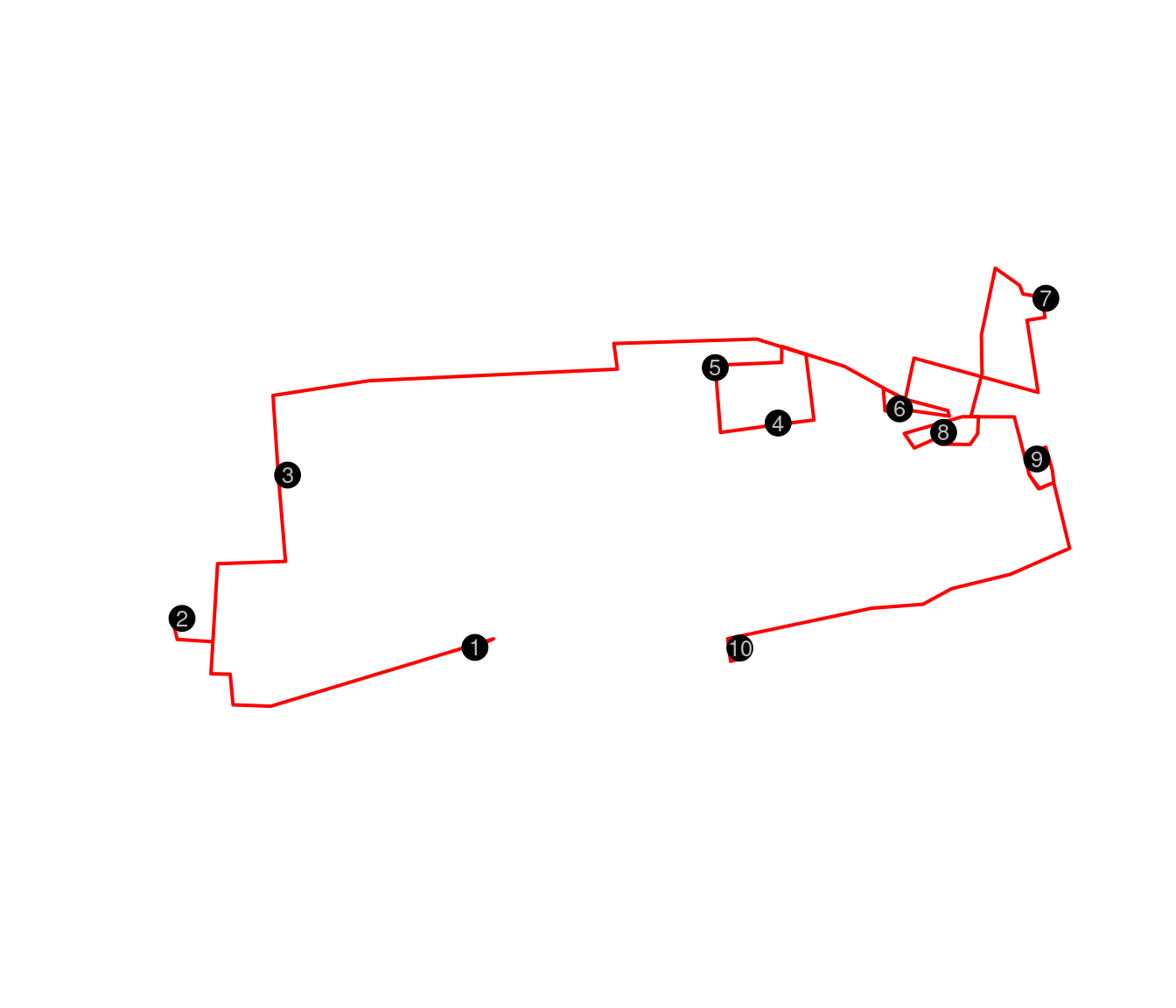
Ruta entre los museos con la optimización AG
In Figure the optimized route shows the route through the streets using OSRM, but without showing the context.
## load packages
library(leaflet)
library(htmlwidgets)
library(webshot)

## we create the map with the route
m <- leaflet(data = sf::st_geometry(ruta1)) %>%
  setView(lng = mean(locs$lon), lat =mean(locs$lat), zoom = 14) %>%
  addTiles() %>%
  addMarkers(lng = locs$lon, lat = locs$lat, popup = locs$id) %>%
  addPolylines()

m
Mapa de los puntos optimizados y con una ruta real gracias al OSRM
## guarda de html to png
#saveWidget(m, "temp.html", selfcontained = FALSE)
#webshot("temp.html",file = "Rplot.png",
#        cliprect = "viewport")
In Figure the optimized route shows the route through the streets using OSRM, but showing the context in an interactive map in html. However, for the purposes of this pdf document, such interaction is not possible.
Conclusion
The process described and outlined in this document shows a feasible solution for creating routes for IPC data collectors in the field. We were able to show that the battery of data management tools that exists, and especially open source programs and software, are an important actor when it comes to creating high-quality innovation, but with a low associated cost. It is absolutely feasible to create route optimization processes with this tool, which requires limited training in the case of training teams of software developers.
It is important to note that, for this problem, the optimized result meets the requirements of being a quality optimization and as shown in the findings of the report “Rutas óptimas para los recolectores del IPC” there is a reduction of 15 % in the travel times of the routes that the data collectors made in previous years.
This algorithm works well when working with no more than 50 points to go. It would be very rare for a data collector to cover more than 15 locations a day during their workday. Typically, that tour takes between 10 and 15 establishments in your work time. Therefore, in order to solve this problem in these terms, the results are convenient in reducing the total time.
On the other hand, and in relation to technical aspects of the process in R, the implementation of Docker and OSRM did not show us great difficulties. While these results are not a top-of-the-line scientific innovation, putting together, combining, and synergizing the processes shown here makes it an innovation. It goes without saying that we take advantage of those who by philosophy make the development of their work available to the public, such as the OSRM project or OSM. Tools that are part of a collaborative and beneficial work scheme for all parties. The free software and open source philosophy community encourages this type of work.
Finally, it should be noted that in this stage we have worked during 2020. However, this year 2021 we are very interested in continuing to study and learn about tools that allow us to package this entire process on a local server of the institution, in order to make available a A tool that allows solving queries to optimize routes for the institution and improve data collection in the field, but perhaps if the project grows over time it can also help and serve the needs of many institutions. Mainly, considering that this tool is not only useful for the National Institute of Statistics (INE-Chile), but also for the ministries, municipalities and especially, to achieve a more precise distribution of social aid and medicines that the population needs in these times of health contingency.
Reference
R Core Team (2020) programming software. A: A language and environment for statistical computing. R Foundation for Statistical Computing, Vienna, Austria. URL https://www.R-project.org/.↩︎
https://github.com/Project-OSRM / osrm-backend↩︎
https : //releases.ubuntu.com/20.10/↩︎
Luxen, D., & Vetter, C. (2011, November). Real-time routing with OpenStreetMap data. In Proceedings of the 19th ACM SIGSPATIAL international conference on advances in geographic information systems (pp. 513-516).↩︎
Copyright © 2021 SIE-INE, Attribution-ShareAlike 3.0 IGO. Contacto rutasoptimas at gmail.com